WEEK 3
Remote sensing data
This is a learning diary of CASA0023 WEEK 3, the lecture presentation is here, and the practical material is here.
1 Summary: lecture
This week focuses on the pre-processing of remote sensing data, including the correction, joining and enhancement of various types of remote sensing data.
1.1 Pre-knowledge
Different sensors
MSS(Multispectral Scanner)RBV(Return Beam Vidicon Camera)
Push broom vs Whisk broom
Whisk broomor spotlight or across track scanners: Mirror reflects light onto 1 detector - LandsatPush broomor along track scanners: several detectors that are pushed along - SPOT, Quickbird
1.2 Corrections
Regression
\[ y_i=\beta_0+\beta_1x_i+\varepsilon_i \]
β0is the intercept (the value of y when x = 0)β1the ‘slope’ the change in the value of y for a 1 unit change in the value of xϵiis a random error term (positive or negative)- if you add all of the vertical differences between the blue line and all of the residuals, it should sum to 0- Any value of y along the blue line can be modeled using the corresponding value of x
Geometric correction
What leads to image distortions
View angle(off-nadir)Topography(e.g. hills not flat ground)Wind(if from a plane)Rotation of the earth (from satellite)
Geometric correction solution
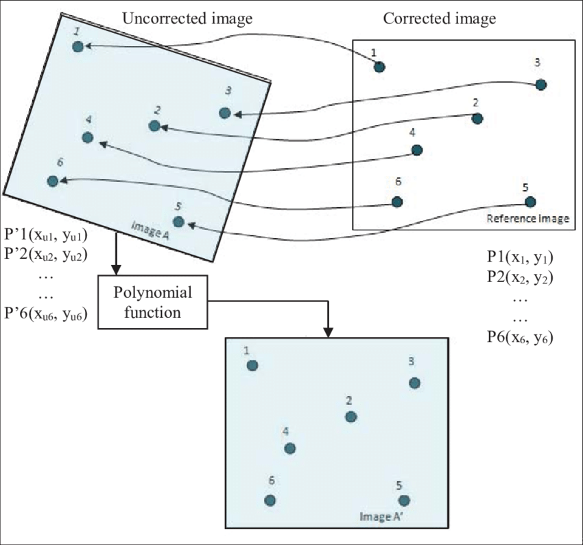
Identify Ground Control Points (GPS) to match known points in the image and a reference dataset
Take the coordinates and model them to give geometric transformation coefficients, linear regression with our distorted x or y as the dependent or independent
Input to output (forward mapping): the issue with this is that we are modelling the rectified x and y which could fall anywhere on the gold standard map (e.g. not on a grid square or at a floating point)Output to input (backward mapping): for every value in the output (gold standard) pixel we can get a value in the original input image. The images are distorted as so might not completely overlap. The goal is to match the distorted image with the gold standard image, so we want the pixels to line up
Plot these and try to minimise the RMSE - Jensen sets a RMSE value of 0.5, typically might add more GCPs to reduce the RMSE (The model with the lowest RMSE will fit best)
RMSE: (observed - predicted (the residual))^2, sum them and divide by number of data points, square root that totalResample methods: Nearest Neighbor, Linear, Cubic, Cubic spline
Atmospheric correction
Necessary and unnecessary atmospheric correction
- Necessary
- Biophysical parameters needed (e.g. temperature, leaf area index, NDVI)
- Using spectral signatures through time and space
- Unnecessary
- Classification of a single image
- Independent classification of multi date imagery
- Composite images (combining images)
- Single dates or where training data extracted from all data
Atmospheric correction in action
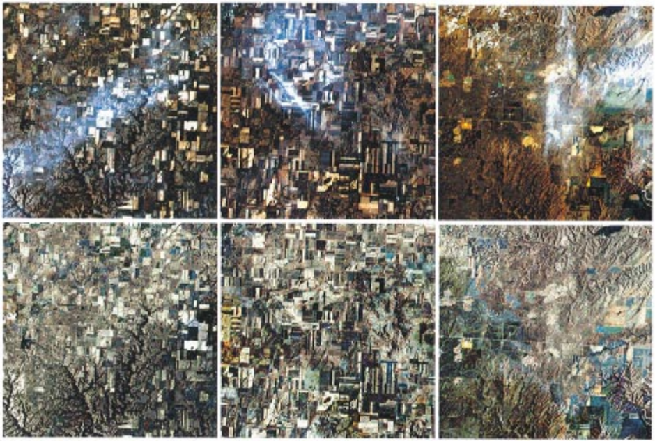
Absorptionandscatteringcreate the haze = reduces contrast of image- Scattering = can create the “adjacency effect”, radiance from pixels nearby mixed into pixel of interest
Atmospheric correction types
- Relative (to something)
Normalize- Normalize intensities of different bands within a single image
- Normalise intensities of bands from many dates to one date
Dark object subtraction (DOS)orhistogram adjustment- Searches each band for the darkest value then subtracts that from each pixel
- Landsat bands 1-3 (visible) have increased scattering vs longer wavelengths
Psuedo-invariant Features (PIFs)- Assume brightness pixels linearly related to a base image
- Regression per band
- Adjust the image based on the regression result
- Here y is the value of our base. To get y we multiply our new date pixel (x) by the coefficient and add the intercept value
- Apply this to the rest of the pixels
- Absolute (definitive)
- Method
- Change digital brightness values into scaled surface reflectance. We can then compare these scaled surface reflectance values across the planet
- We do this through atmospheric radiative transfer models and there are many to select from
- However, nearly all assume atmospheric measurements are available which are used to “invert” the image radiance to scaled surface reflectance
- The scattering and absorption information comes from atmopshierc radiative transfer code such as MODTRAN 4+ and the Second Simulation of the Satellite Signal in the Solar Spectrum (6S), which can now be used through python - called
Py6S
- Absolute Data requirements
An atmopsheric model(summer, tropical): usually you can select from the toolLocal atmopsheric visibility: from a weather station, like airportsImage altitude
- Absolute Tools
ACORN: Atmopsehic CORection NowFLAASH: Fast Line of-sight Atmopsheric AnalysisQUAC: Quick Atmopsheric CorrectionATCOR: The ATmospheric CORrection programSMAC: Simplified Model for Atmospheric Correction (SMAC)
- Method
- Empirical Line Correction
- We can go and take measurements in situ using a field spectrometer, this does require measurements at the same time as the satellite overpass
- Then use these measurements in linear regression against the satellite data raw digital number
Orthorectification / Topographic correction
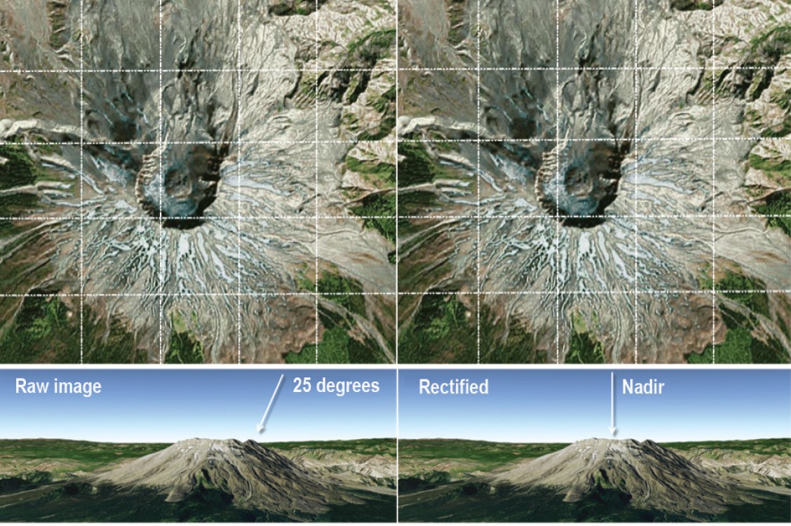
A subset of georectification
Georectification= giving coordinates to an imageOrthorectification= removing distortions… making the pixels viewed at nadir (straight down)
Requires
Sensor geometryAn elevation model
Software / formulas to do this
- Jensen covers the following
formulas: Cosine correction, Minnaert correction, Statistical Empirical correction, C Correction (advancing the Cosine) Software: QGIS, SAGA GIS, R package topocorr, R package RStoolbox
Solar location
Solar azimuth= compass angle of the sun (N =0°) 90° (E) at sunrise and 270° (W) at sunsetSolar zenith= angle of local zenith (above the point on ground) and sun from vertical (90° - elevation)
Radiometric calibration
- Sensors capture image brightness and distributed as a
Digital Number (or DN)- allows for efficient storage but has no units - Spectral radiance is the amount of light within a band from a sensor in the
field of view (FOV), it is independent of the sensor, measured in Watts (power or light here) - DN to spectral radiance =
radiometric calibration Sensor calibration= the relationship between Gain and Bias are usually provided but we can calcaulte them
Radiance: refers to any radiation leaving the Earth (i.e. upwelling, toward the sensor- Might also be called Top of Atmosphere (TOA) radiance
- How much light the instrument sees in meaningful units but still have effects of: Light source, atmosphere and surface material
- We can remove the effects of the light source to generate Top of Atmosphere reflectance but usually this is combined within the radiance to reflectance step
Irradiance: is used to describe downwelling radiation reaching the Earth from the sunDigital number (DN)- Intensity of the electromagnetic radiation per pixel
- Pixel values that aren’t calibrated and have no unit
- Have light source
- Effects of sensor + atmosphere + material
- Values range from 0 - 255 (Lansat 5) = 8 bit or 0 - 65536 Landsat 8 (12 bit)
Reflectance: We need to account for atmospheric and illumination effects to create reflectance. BUT this typically doesn’t deal with shadows and directional effects (e.g. viewing angles) = apparent reflectance However, this is often called reflectance- Reflectance is a property of a material (e.g. reflectance of grass is a property of grass)
- The issue with radiance is that is contains physical properties AND is dependent on the light source
Hemispherical reflectance: all of the light leaving the surface goes straight to the sensor (nothing is intercepted or at an angle)Path radiance: radiance reflected above the surface (e.g. scattering)Atmospheric attenuation: absorption of EMR due to materials in atmosphere (e.g. water vapour)Local: specific to pixel- `Neighbourhood: pixels within a range (nearby)
1.3 Data joining and enhancement
Joining data sets
- This is termed “Mosaicking” in remote sensing - but it’s not much different to merging in GIS
- In Remote Sensing we usually
featherthe images together - This creates a seamless mosaic or image(s)
- The dividing line is termed the
seamline - We have a base image and “other” or second image
How to join data sets
Standardization(dividing the SR value by a maximum value per band) andnormalization(divide the standarised value by the sum of values across all bands) applied to each image- Undertake further relative
radiometric normalization Classifyeach image aloneCalculateother metrics from the image
Image enhancement
Contrast enhancement
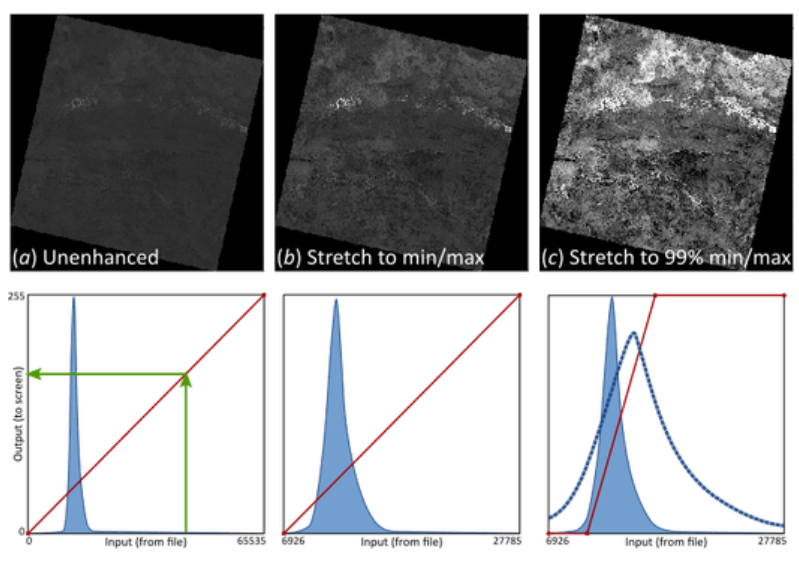
Minimum - MaximumPercentage LinearandStandard DeviationPiecewise Linear Contrast Stretch
Ratio
Band ratioingmeans dividing the pixels in one band by the corresponding pixels in a second band.- Example: Normalized Burn Ratio = (NIR - SWIR) / (NIR + SWIR)
- In Landsat 4-7, NBR = (Band 4 – Band 7) / (Band 4 + Band 7)
- In Landsat 8-9, NBR = (Band 5 – Band 7) / (Band 5 + Band 7)
Filtering
Low passorlow frequency(averages the surrounding pixels)High passorhigh frequency- enhance local variationsEdge enhancement
PCA (Principal Component)
- Transform multi-spectral data into uncorrelated and smaller dataset
- Has most of the original information
- Reduces future computation “dimensionatliy reduction”
- The first component will capture most of the variance within the dataset
- In R this is from the RStoolbox packagerasterPCA()
- PCA example, multi-date PCA - bands from both time points are combined into one image, then PCA
Texture
- Images just use tonal (spectral) data not texture
Texture: spatial variation of gray valuesFirst order (occurrence): use counts or occurrencesSecond order(co-occurrence): relationship between pixel pairs “a function of both the angular relationship and distance between two (or kernel) neighboring pixels”
Fusion
Image fusion is where data from multiple sensors / sources is fused together
- Pan sharpen
- Data Fusion
2 Summary: practical
This week’s practical will consist mainly of the following:
- Introduction and access to Landsat data
- A deeper understanding of atmospheric correction and how it works in practice
- Introduction to the principles of Radiance (or DN) to Reflectance
- Practical exercises in image joining
- A deep understanding of image enhancement and how it works in practice
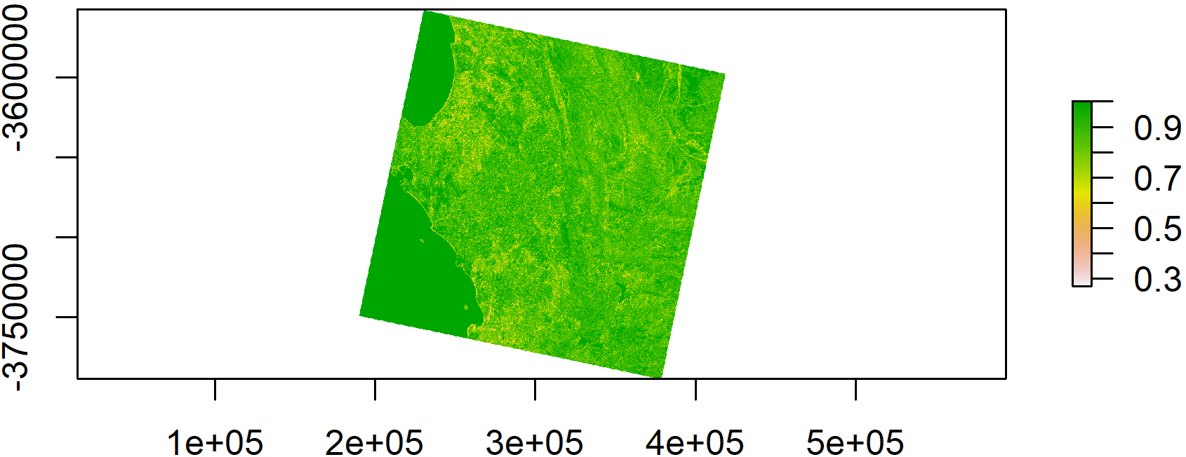
For this week’s practical I chose to follow the guidance using Landsat data from Cape Town. I used R to do atmospheric corrections, merging, data enhancement and other operations on the data. Through practical, I gained a better understanding of remote sensing data pre-processing and was able to apply this to my workflow in R. Combined with the previous term’s CASA0005 course, I can now use R to analyse more types of data.
3 Application
This week, the main focus was on the correction, joining and enhancement of remote sensing images, mostly applied to pre-processing before analysis, but remote sensing image enhancement has a wider range of applications.
3.1 Applications of remote sensing image enhancement
Remote sensing image enhancement refers to the improvement of the quality and information of remote sensing images through some technical means to make them more suitable for human vision or subsequent analytical processing. Remote sensing image enhancement can be applied to the following areas:
Contrast enhancement: By adjusting the grey level of a remotely sensing image, the contrast of the image is increased to make it clearer and brighter. Contrast enhancement can be done using methods such as histogram stretching, histogram equalisation and segmented linear stretching.
Band ratioing: Extracts specific information from remote sensing images, such as vegetation indices, water indices, soil indices, etc., by calculating the ratio between different bands. Band ratios can be calculated using methods such as band arithmetic and band combination.
Filtering: Remove noise or enhance edges and textures in an image by convolving the remote sensing image in the spatial or frequency domain. Filtering can use methods such as smoothing filtering, sharpening filtering and edge detection filtering.
Principal component analysis (PCA): By applying orthogonal transformations to multiple bands of remote sensing images, the main information in the image is extracted and the redundancy and correlation of the data is reduced. Principal component analysis can use statistical methods or methods such as wavelet transform.
Texture: Describes the surface roughness or structural features in an image by calculating the grey scale variation within a region of the remotely sensed image. Texturing can use methods such as grey level co-occurrence matrix, grey level distance matrix, grey level gradient matrix, etc.
Fusion: Increasing the spatial or spectral resolution of an image and increasing the amount of information in the image by combining remote sensing images from different sources or at different resolutions. Fusion can be done using methods such as HIS transform, wavelet transform, multi-resolution analysis, etc.
3.2 Application case
PCA‐based land‐use change detection and analysis using multitemporal and multisensor satellite data , Sourse: Deng et al. (2008)
Remote‐sensing change detection based on multitemporal, multispectral, and multisensor imagery has been developed over several decades and provided timely and comprehensive information for planning and decision‐making. In practice, however, it is still difficult to select a suitable change‐detection method, especially in urban areas, because of the impacts of complex factors.
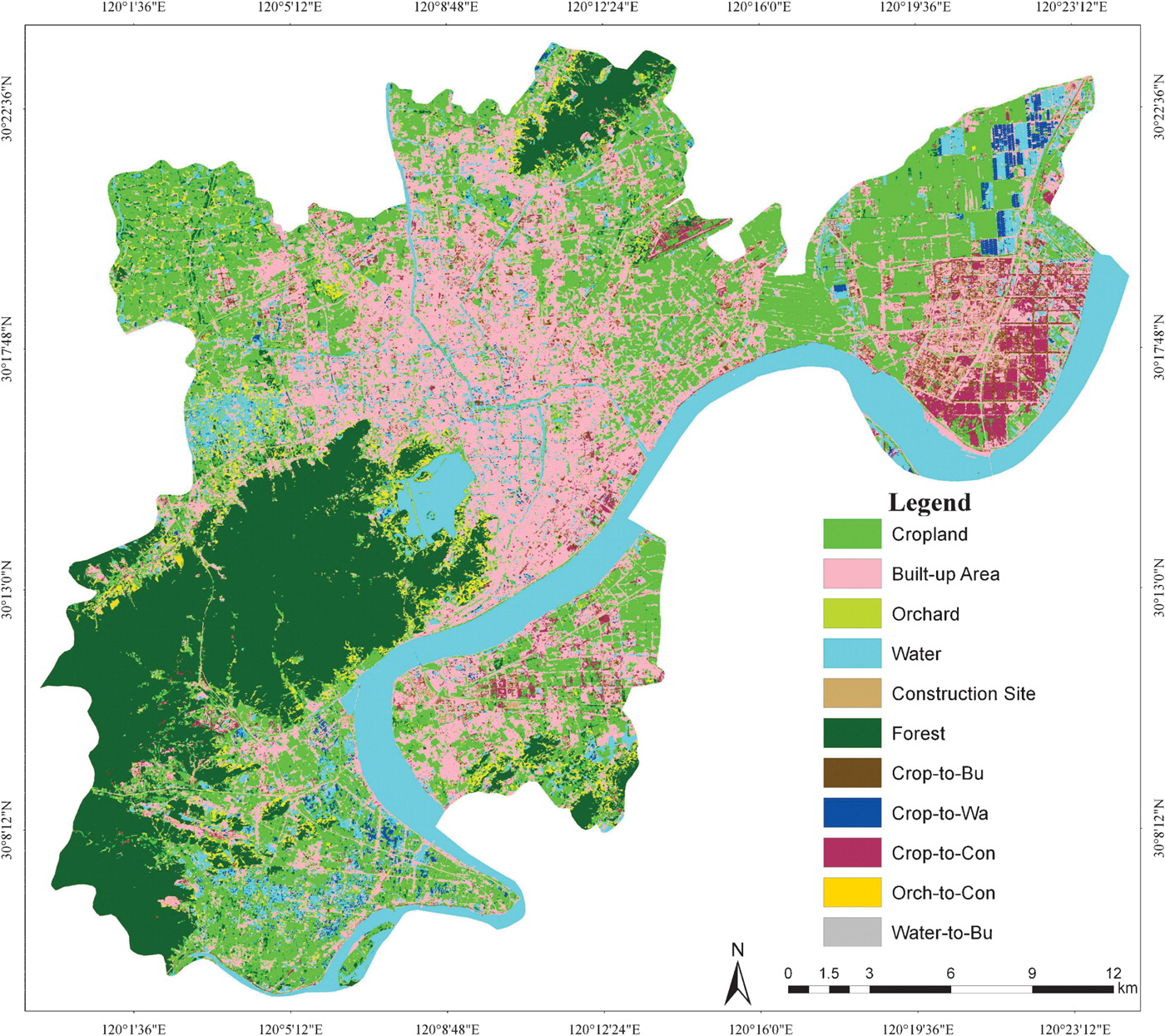
This paper presents a new method using multitemporal and multisensor data (SPOT‐5 and Landsat data) to detect land‐use changes in an urban environment based on principal‐component analysis (PCA) and hybrid classification methods. After geometric correction and radiometric normalization, PCA was used to enhance the change information from stacked multisensor data. Then, a hybrid classifier combining unsupervised and supervised classification was performed to identify and quantify land‐use changes. Finally, stratified random and user‐defined plots sampling methods were synthetically used to obtain total 966 reference points for accuracy assessment.
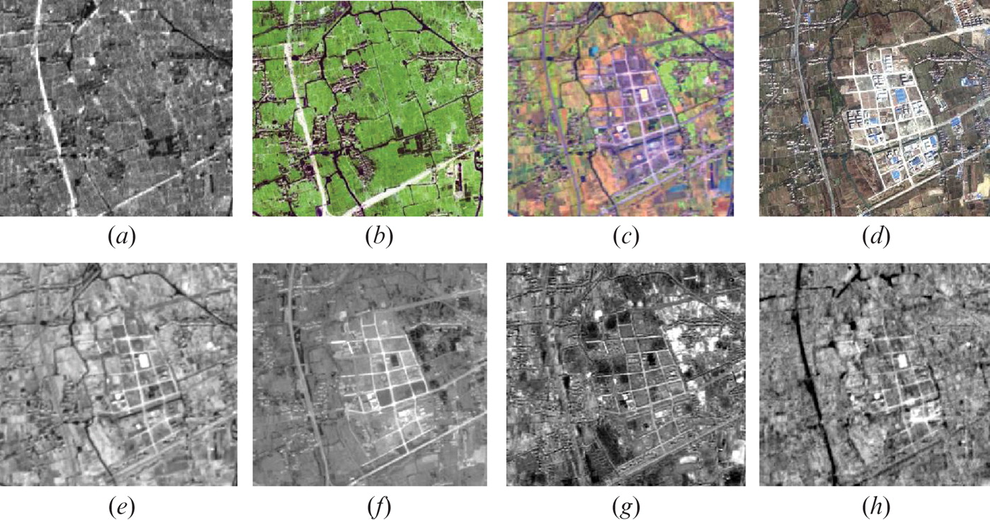
Although errors and confusion exist, this method shows satisfying results with an overall accuracy to be 89.54% and 0.88 for the kappa coefficient. When compared with the post‐classification method, PCA‐based change detection also showed a better accuracy in terms of overall, producer’s, and user’s accuracy and kappa index. The results suggested that significant land‐use changes have occurred in Hangzhou City from 2000 to 2003, which may be related to rapid economy development and urban expansion. It is further indicated that most changes occurred in cropland areas due to urban encroachment.
3.3 Case comments
Advantages or contribution
- Flexible classification strategies: The hybrid classification approach allows the authors to combine the accuracy of supervised classification methods while taking advantage of the automation of unsupervised classification methods. This flexibility allows the method to be better adapted to different types of land use change scenarios.
- PCA-based feature extraction: By combining multi-temporal and multi-sensor data into a single Principal Component Analysis (PCA) model, the authors are able to extract more meaningful features that help distinguish between changing and non-changing areas. This approach has advantages in dealing with high-dimensional data and reducing data redundancy.
- Correction and radiation normalisation: This paper corrected and radiation normalised the data prior to analysis, which helped to reduce errors due to sensor differences, variations in atmospheric conditions and land cover type, thus improving the accuracy and reliability of the results.
Disadvantages or potential
- Limitations of Principal Component Analysis (PCA): While PCA is able to extract and enhance variation information from multi-sensor data, it may not be able to completely eliminate noise and other non-target factors. In addition, PCA may have limitations in handling non-linear data, which may lead to inaccurate detection results.
- Limitations of sensor data: SPOT-5 and Landsat data were used in this paper. While these data sources are of value in land cover change detection, they may not capture the detailed information that finer spatial resolution and higher spectral resolution can provide. In addition, these data sources may be affected by issues such as cloud occlusion, atmospheric interference and timing inconsistencies.
4 Reflection
This week I learnt the principles and methods of correcting, joining and enhancing remotely sensed images and understood how to pre-process remotely sensed data. Although most of the data we acquired had already been pre-processed, this knowledge gave me a better understanding of how to apply remote sensing images to the actual analysis and what could cause errors and whether further processing was needed. In addition, the study of remote sensing image enhancement has taught me more about remote sensing data analysis methods and principles in a deeper way.
However, not all data pre-processing can be perfectly accurate, errors are allowed but need to be controlled according to the actual situation. Also, in practice, some R packages are no longer available due to version updates. This is a common problem in data analysis and can be solved by downloading a lower version of the package or replacing it.