WEEK 1

An Introduction to Remote Sensing

This is a learning diary of CASA0023 WEEK 1, the lecture presentation is here, and the practical material is here.

1 Summary: lecture

This week’s content focuses on an introduction to basic information on remote sensing and Electromagnetic radiation (EMR).

1.1 Remote sensing

Definition

NASA defines remote sensing as acquiring information from a distance, interchangeable used with Earth Observation or EO.

Data acquisition

This is achieved through sensors mounted on a platform, e.g. satellites, planes (aerial imagery), drones, phones, free standing on the ground or sea (with hand held devices), there are more than 150 satellites in orbit carrying sensors.

Advantages

Mass of data: satellites collect data on the same points on Earth every day to every 16 days
Frequency of update and less reliance on authorities (e.g. London Atlas)
More free resources to process large volumes of data (e.g. Google Earth Engine)

Types of sensor

Passive sensor

Use energy that is available
Don’t emit anything
Usually detecting reflected energy from the sun
Energy is in electromagnetic waves…
Such as: Human eye, camera, satellite sensor

Active sensor

Have an energy source for illumination
Actively emits electormagentic waves and then waits to receive
Such as: Radar, X-ray, LiDAR

1.2 Electromagentic waves

Terms

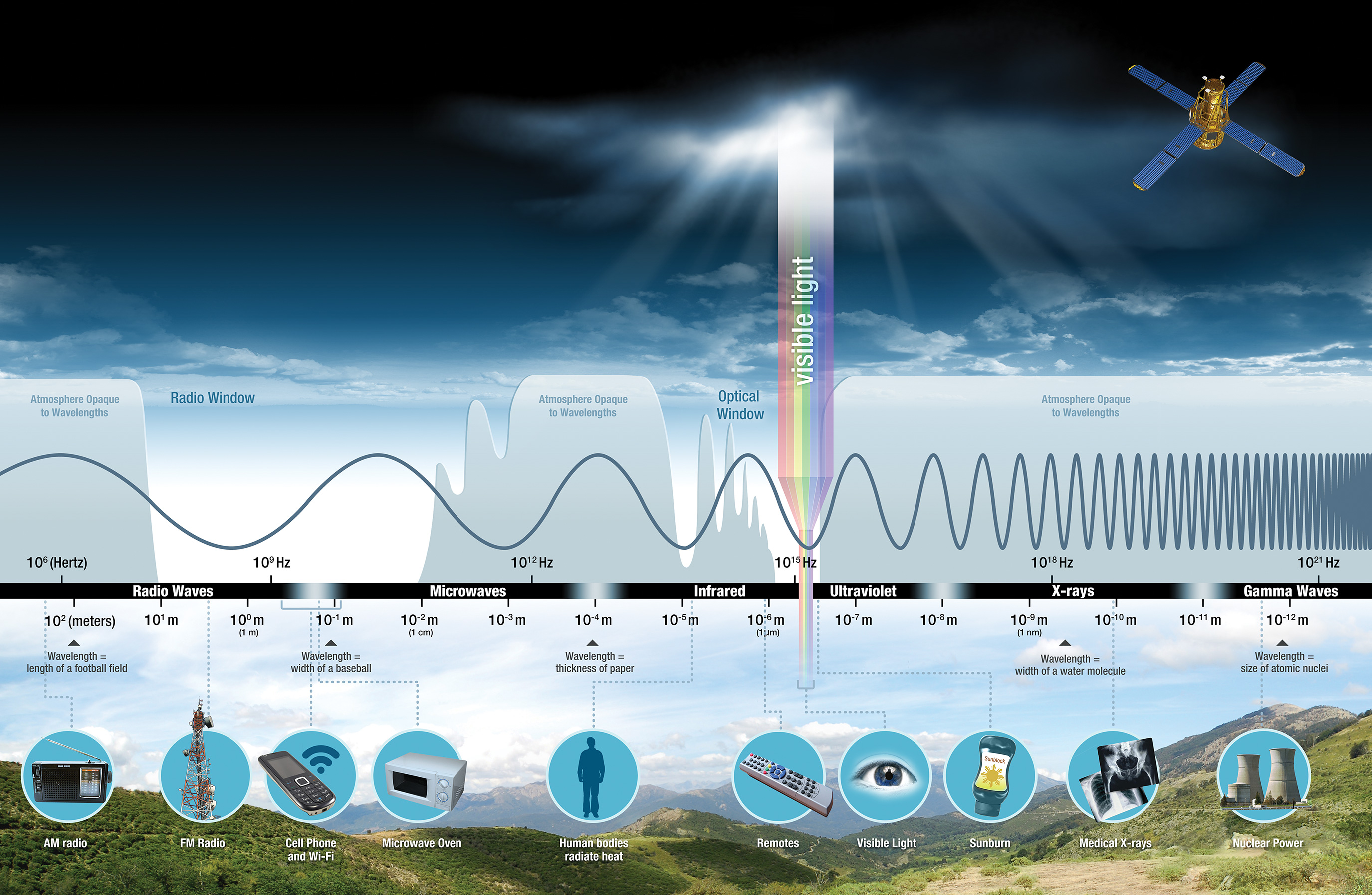
Waves of an electromagnetic field, travel through space and carry radiant energy = Electromagnetic radiation (EMR). Waves are part of the EMR spectrum.
Energy carried by EMR waves = radiant energy
Energy per unit of time = radiant flux
Energy from the sun = incoming short wave radiation or shortwave radiation
Energy (solar power) from the sun per unit area per unit time (from electromagnetic radiation) = solar irradiance (per unit time - flux)
Energy leaving a surface per unit area per unit time = Exitance (emittance) (per unit time - flux)
Flux means time here.

Electromagnetic radiation (EMR)

EMR has both electric and magnetic fields, propagates (moves) as waves: c = vλ

c = velocity of light 3 x 10^8 meters per second
v = frequency, rate of oscillation
λ = wavelength, distance between two crests

EMR isn’t automatically reflected. It experiences a number of changes prior to hitting the sensor

Surface: Energy being absorbed by the surface and being transmitted through the surface
Atmospheric: Energy can be scattered by particles in the atmosphere

1.3 Interacting with Earth’s surface

Atmospheric scattering

Rayleigh = particles are very small compared to the wavelength
Mie = particles are the same size compared to the wavelength
Non selective = particles are much larger than the wavelength

Synthetic Aperture Radar (SAR)

Radar collects at longer wavelengths than optical sensors - pass through clouds that have smaller particle sizes (wavelength dictates how far it can penetrate into medium)
Has it’s own bands - e.g. P, L, S, C, X, Ku, K
Collects data at night

Bidirectional Reflectance Distribution Function (BRDF)

View (e.g. sensor) and illumination (e.g. sun) angles can change
Energy being reflected from the surface that is smooth or diffuse

Polarization

Definition

Applicable to Radar: Electromagnetic waves are polarized and the direction depends on the oscillation of the electromagnetic field. When they are reflected from the surface the waves can be linked to surface properties - roughness, shape, orientation, moisture, salinity, density.

Different ploarizations

Single polarization: same polarization transmitted and received = 1 horizontal (or vertical)
Dual polarization: One sent, different one received = transmits and receives both horizontal and vertical
Quad polarization: system can transmit and receive four types = emitted in horizontal (H) and received in horizontal (H)

1.4 Remote sensing data

Data formats

band interleaved by line (BIL)
band sequential (BSQ)
band interleaved by pixel (BIP)
GeoTIFF (most common)

Four resolutions

Spatial = the size of the raster grid per pixel (e.g. 20cm or 30m)
Spectral = the number of bands it records data in…more soon
Temporal = the time it revisits (e.g. daily, every 7 days, on demand)
Radiometric = identify differences in light or reflectance, in practice this is the range of possible values.

Spectral resolution. Source: NASA Science

Type of orbit

geosynchronous orbit (GSO) = satellite matches the Earth’s rotation
geostationary orbit = holds same position, usually only for communications but some sensors are geostationary.

2 Summary: practical

This week’s practical will consist mainly of the following:

Acquisition and reading of remote sensing data

The specifics of processing remote sensing data using SNAP and R

Methods for viewing the spectra of remote sensing data and comparing spectral features

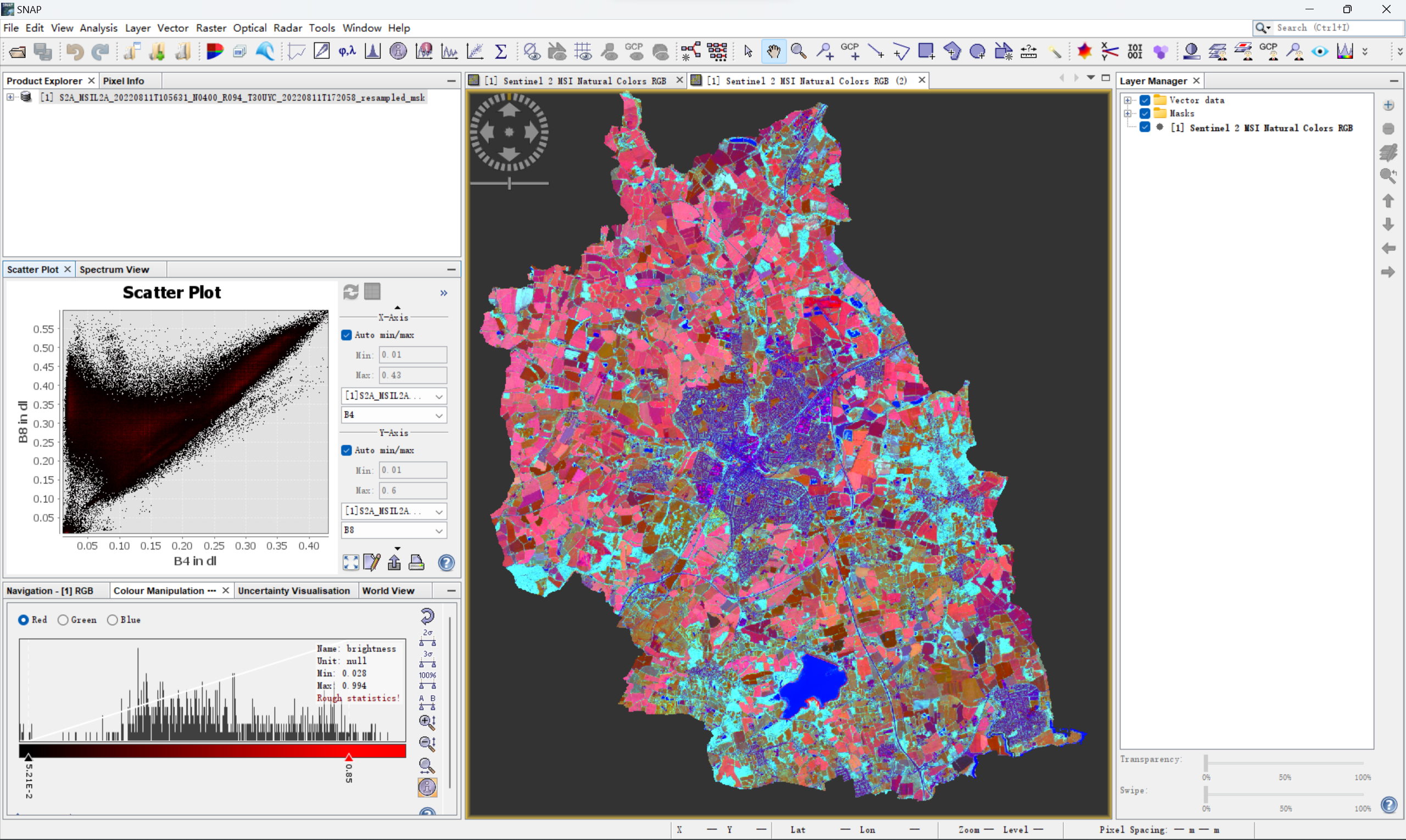
For this week’s practical I chose Chelmsford, a city in the north-east suburbs of London, as my study area. I also followed the practical’s instructions to operate on remote sensing images within its administrative area. Through this practical I became familiar with the use of SNAP and the remote sensing related package of R. I also learnt about some of the features of remote sensing imagery, such as spectral features, through these operations.

3 Application

This week’s lecture is mainly about the basic knowledge of remote sensing and Electromagnetic radiation (EMR), so I would like to introduce some of the remote sensing applications based on spectral characteristics.

3.1 Remote sensing applications based on spectral features

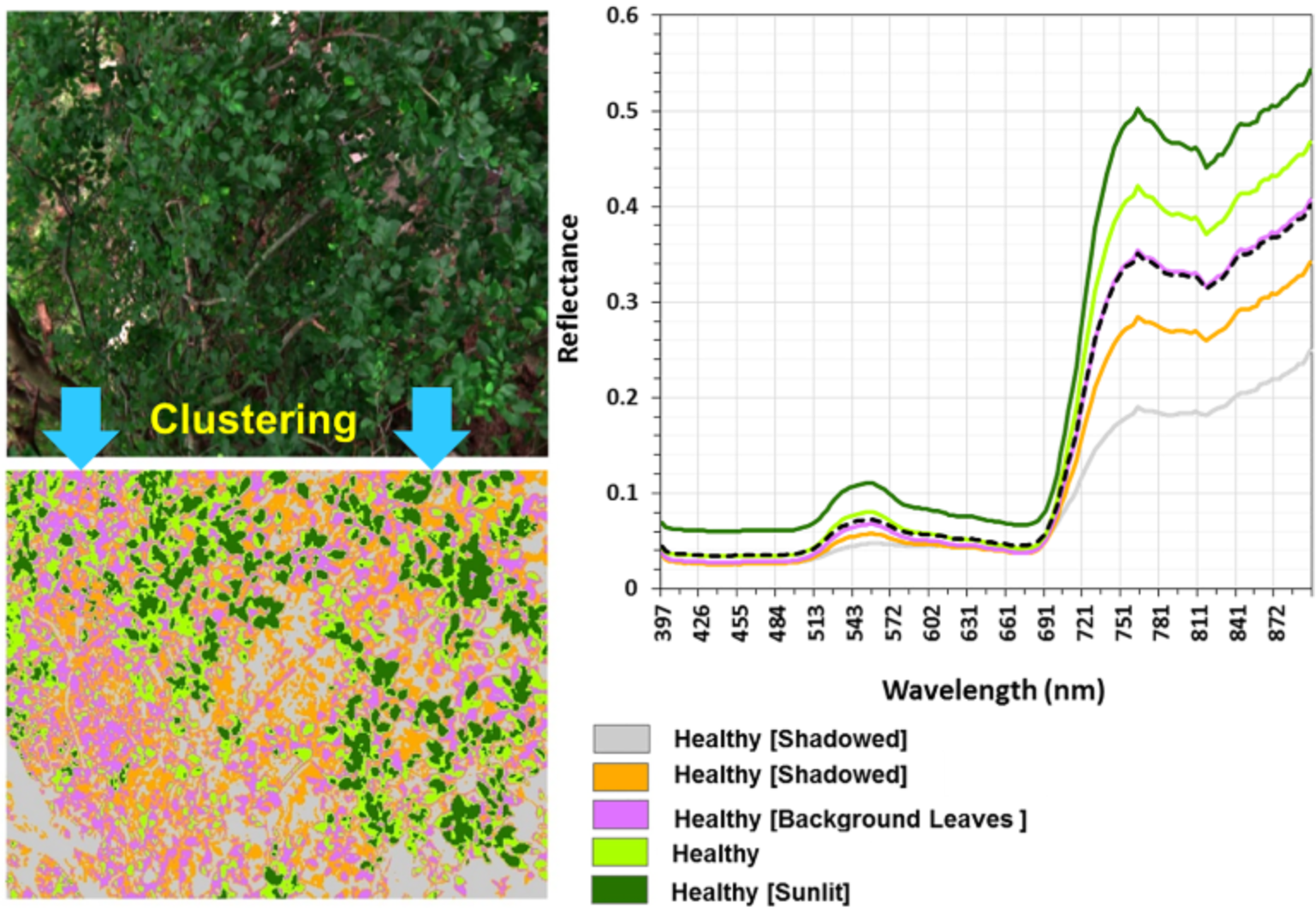
Remote sensing uses spectral features to identify, classify and analyse a variety of features on the surface or in the atmosphere. Remote sensing has many applications using spectral features：

In the field of agriculture, the spectral characteristics of vegetation can be used to monitor the growth of crops, damage, yield prediction, etc.
In the field of environmental, the spectral characteristics of water bodies, soil and atmosphere can be used to monitor water quality, soil types, pollutant types and concentrations, etc.
In the field of geology, the spectral characteristics of rocks, minerals, etc. can be used to detect mineral resources, geological formations, seismic activity, etc.
In the field of urban planning, the spectral characteristics of buildings, roads, etc. can be used to extract urban spatial information, assess the level of urban development and influencing factors, etc.

The specific application methods of remote sensing based on spectral features in the field of urban planning are mainly as follows:

Using remote sensing images to obtain information on the current situation of land use, analyse the structure and spatial distribution characteristics of urban land use, and provide basic data for urban planning.
Using remote sensing images for urban ecological environment evaluation, monitoring urban heat island effect, air quality, tree health, water quality and other environmental indicators, and providing ecological guarantee for urban planning.
Use remote sensing imagery for urban construction change monitoring, identifying the impact of urban construction activities on land use, and providing dynamic management for urban planning.

3.2 Application case

Sourse

Characterizing and classifying urban tree species using bi-monthly terrestrial hyperspectral images in Hong Kong , Sourse: Abbas et al. (2021)

Urban trees exhibit a wide range of ecosystem services that have long been unveiled and increasingly reported. The ability to map tree species and analyze tree health conditions would become vividly essential. Remote sensing techniques, especially hyperspectral imaging, are being evolved for species identification and vegetation monitoring from spectral reponse patterns.

An example of image clustering and corresponding spectral signatures of classes. The shadow class in grey represents canopy shadow and/or branches, and the shadow class in orange indicates shaded leaves.

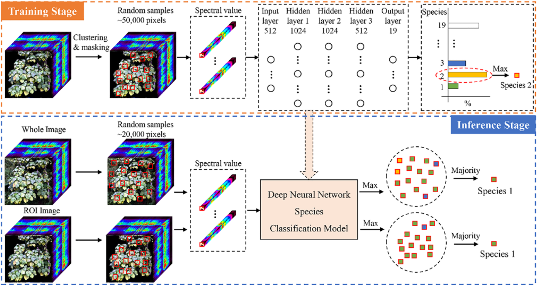
In this study, a hyperspectral library for urban tree species in Hong Kong was established comprising 75 urban trees belonging to 19 species. 450 bi-monthly images were acquired by a terrestrial hyperspectral camera (SPECIM-IQ) from November 2018 to October 2019. A Deep Neural Network classification model was developed to identify tree species from the hyperspectral imagery with an overall accuracy ranging from 85% to 96% among different seasons. Representative spectral reflectance curves of healthy and unhealthy conditions for each species were extracted and analyzed. This can be used to identify urban trees and monitor their health.

The overall workflow of species classification framework using the Deep Neural Network modelling.

3.3 Case comments

Advantages or contribution

A hyperspectral library for urban tree species in Hong Kong was established , and trees were classified and detected with high accuracy, which could be a valuable resource for future research in Hong Kong or similar environments.
Hyperspectral phenology models were developed using deep neural network classification models to optimise data acquisition and improve accuracy in monitoring tree health, which provides experience in the field of machine learning of remote sensing images.

Disadvantages or potential

Hyperspectral image acquisition cost and processing complexity: Acquisition and processing of hyperspectral images may be more costly and complex compared to other remote sensing techniques, and may face cost issues in actual applications.
Data set limitations: The study focuses on urban trees in Hong Kong and may not be directly applicable to other regions or cities with different ecological conditions. Expanding the study to include a wider range of geographical and ecological conditions would make the results more generalisable.

4 Reflection

During this week I have learnt about the basics of remote sensing and Electromagnetic radiation (EMR), which has greatly broadened my horizons when researching urban. Due to limited data collection facilities, detailed urban datasets (e.g. traffic flow data, mobile phone signalling data, etc.) are only available for main cities in developed areas, which makes many studies not reproducible in a wide range of non-developed or small cities. However, the extensive coverage of remote sensing data compensates well for this shortcoming, and the variety of data collected through the rich diversity of sensors can be of great help in urban (or regional) analysis.

However, there are some limitations to remote sensing data at the level of accuracy and price. On the one hand, there is relatively little high-precision remote sensing data for inner-city scale studies, and on the other hand, high-precision data often leads to huge costs, which in practice can lead to some technologies not being implemented.